Fuzzy Sets
Fuzzy Sets in Hydrologic Modeling: HFAM Simulation Algorithms
The conviction that traditional methods of systems analysis are unsuited for dealing with systems in which relations between variables do not lend themselves to representation regarding differential or difference equations is what motivated my paper on fuzzy sets (1965).
— Lofti Zadeh
If we were seeking a real world problem that is inherently messy, where mathematical functions are difficult to apply, hydrologic modeling for surficial hydrologic processes would be an excellent example. Surficial hydrologic processes (at or near the land surface) depend on topography, vegetation, and soil properties including soil moisture – and on rainfall patterns and intensity, potential evapotranspiration, air temperatures, solar radiation, winds, and dewpoints. Each of the variables listed changes in either space or time and many change in both space and time. Nonetheless, we want to calculate hydrologic processes in this real world environment.
Hydrologic models are useful only to the degree that they represent processes in the world.
Methods for dealing with surficial hydrologic processes are:
A) solve for key processes like infiltration rate at many points on the watershed surface. When different permeabilites, moisture storages, etc. are used at each point on the watershed surface, point to point variability in processes should create continuously variable, or physically realistic, aggregate watershed behavior.
B) use fuzzy sets or continuous functions to interrelate variables in hydrologic process calculations and model aggregate behavior directly.
Methods for dealing with surficial hydrologic processes
Solve for key processes like infiltration rate at many points on the watershed surface. When different permeabilities (e.g. moisture storages) are used at each point on the watershed surface, point to point variability in processes should create continuously variable, or physically realistic, aggregate watershed behavior.
Use fuzzy sets or continuous functions to interrelate variables in hydrologic process calculations and model aggregate behavior directly.
The original Stanford Watershed Model published in 1962 and 1966 used fuzzy sets. Professor Lotfi Zadeh’s paper on “Fuzzy Sets,” published in the journal Information and Control in 1965 {Zadeh, L. A. “Fuzzy Sets” Information and Control 8(1965): 338-53}, was not read at Stanford by the hydrology/hydraulics students at that time. Dr. Zadeh was then Chairman of the Dept. of Electrical Engineering at the University of California, Berkeley.
However, using fuzzy sets and continuous functions in hydrologic algorithms in the Stanford Model came from similar reasoning: It is illogical to have thresholds in modeling where, for example, the surface runoff changes from 0 to 100 percent when the rainfall intensity increases by 0.01 inches per hour.
Figure 1
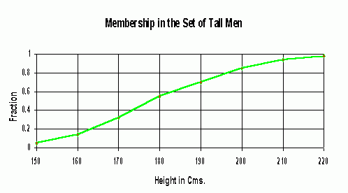
Figure 1 is an example of a fuzzy set of “tall men,” and shows the degree of membership in the set of “tall men,” versus “not tall men” { Cox, E. “The Fuzzy Systems Handbook”, AP Professional, Academic Press Inc. (Harcourt Brace & Company), New York, 1994 }.

Figure 2
Figure 2 shows the percent of infiltrating water captured by the lower zone soil moisture storage versus the lower zone soil moisture storage ratio in the Stanford Watershed Model ( HFAM and HSPF use the same function). The Stanford Model utilized a similar function for the capture of lateral runoff in the upper zone soil moisture storage.
In addition to explicit fuzzy sets, the Stanford/HSPF and HFAM models’ algorithms create fuzzy sets implicitly:

Figure 3
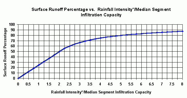
Figure 3 shows a land segment infiltration rate as a fraction of rainfall intensity versus the rainfall intensity* and median infiltration capacity ratio in HFAM. Figure 3 is an internal model result, so it requires definitions. Rainfall intensity* matches rainfall intensity only when interception storage is full. Surface runoff percentage is an assignment to the surface runoff flow path, but water on this flow path can still be captured by near surface storage (upper zone storage) before it enters a stream channel.

Debate on the merits of approaches A or B above is likely to continue in hydrology, just as the debate about fuzzy sets continues in systems analysis.
To compare A and B, we need to define the problem being solved. In A, a solution for processes is made at a point on a watershed, and this solution is extended to areas surrounding the point. If solutions at 1000 points are used in a 100 sq. km. watershed, each solution is applied to 0.1 sq. km. of the watershed surface. The result is called a “distributed” model.
In B, the watershed surface is idealized, by creating “land segments.” Fuzzy sets are used within each land segment to create an aggregate behavior for the land segment.
In HFAM (common with HSPF and the Stanford Models) one land segment has one set of meteorological time series and has unique physical characteristics (e.g. land slope and elevation). Although HFAM may use an arbitrarily large number of land segments and the model is “distributed,” ten to twenty-five land segments would typically be used in a 100 sq. km. watershed rather than 1000. Continuous functions or fuzzy sets are used to represent point-to-point process variability within HFAM land segments.
So far as the laws of mathematics refer to reality, they are not certain. So far as they are certain, they do not refer to reality.
— Albert Einstein
Some comparisons between approaches A and B are as follows:
In A, when soil properties at a point are defined, a numerical solution for infiltration rate at a point is calculated.
This creates the step function or threshold for infiltration shown in Figure 4: The infiltration rate at a point is independent of rainfall intensity. This point solution applied to the land surrounding the point, which may be a fraction of a sq. km. to many sq. kms.
How many point solutions are needed within a watershed to represent the aggregate behavior of watershed lands?
Soil structure, together with areal variability in topography and vegetation, limits the direct use of infiltration functions to areas beyond a point. This is why thresholds as in Figure 4 are a problem.
Keith Beven, for a Symposium on Preferential Flow, writes “soil is not a simple porous medium . . . but has been subject to various physical, chemical, and biological processes that develop ‘structure’ – larger voids that allow flowing water to bypass parts of the soil matrix” {Preferential Flow, Proceedings of the National Symposium, Am. Soc. of Agricultural Engrs., December 1991, Chicago, Illinois}. Field measurements of infiltration rates often show significant variations, even within areas of 100 x 100 meters.
Expanding the number of points in a watershed in approach A (so points may represent only 0.01 sq. km. instead of 0.1 sq. km.) make the problem of model setup and parameter definition and calibration more challenging. Soil properties are needed at each point. Separate meteorological time series, vegetation and topographic parameters for each point may also be needed.
In approach A, an aggregate hydrologic behavior is expected to emerge from solutions at some points within a watershed. Relationships between modeling parameters, like permeability at solution points and the aggregate hydrologic behavior shown in Figures 2 and 3 are not available.
In B, algorithms are specifically designed to represent aggregate hydrologic processes within heterogeneous areas – the land segments. Algorithms deal with membership in sets (i.e. the percent or fraction of a moisture flux that enters soil moisture storage as soil moisture changes). Abrupt thresholds are avoided.
The world of math does not fit the world it describes. The two worlds differ, one artificial and the other messy.
— Bart Kosko
Fussy sets, or the use of continuous functions in complex systems, has been criticized as a “less scientific” than approach A. Fuzzy logic proponents respond by saying that the bias in modern science is for black-white mathematical logic and that problems that do not yield to these classical methods of solution are ignored.
The “less scientific” critique is valid if differential equations or other mathematical tools can be found that adequately represent or model hydrologic processes in the field (modeling processes in a laboratory setting is a different problem). When adequate mathematical tools are not available for complex systems, or when complexity overwhelms the available mathematical tools, there are advantages to fuzzy sets. The Stanford Watershed Model relationship between soil moisture storage indices and aggregate model behavior within land segments, in Figure 2, is clear. This relationship can be used to advantage in model calibration. The number of model parameters used in calibration is also tends to be less, and calibration with fewer parameters is easier.
When adequate mathematical tools are not available for complex systems, or when complexity overwhelms the available mathematical tools, there are advantages to fuzzy sets.
The Stanford Watershed Model relationship between soil moisture storage indices and aggregate model behavior within land segments (Figure 2) is clear. This relationship can be used to advantage in model calibration. The number of model parameters used in calibration also tends to be less, and calibration with fewer parameters is easier.
With HFAM, a model user may choose to make any number of land segments within a watershed to account for variations in precipitation, temperature, vegetation, soils, and more. When these characteristics are accounted for, land segments need not be further sub-divided to model aggregate hydrologic behavior. Aggregate hydrologic behavior is included in HFAM algorithms.
Fuzzy systems models are now being widely applied for analysis of complex non-linear systems.
Kosko, Bart, Fuzzy Thinking: The New Science of Fuzzy Logic, Hyperion, New York , 1993
McNeill, Daniel and Paul Freiberger, Fuzzy Logic: The Discovery of a Revolutionary Computer Technology, Simon and Schuster , New York , 1993
Zadeh, Lotfi. Outline of a New Approach to the Analysis of Complex Systems and Decision Processes, IEEE Transactions on Systems, Man and Cybernetics, SMC-3(1), January 1973.
Kosko, Bart, Neural Networks and Fuzzy Systems, Prentice-Hall Inc., 1992


